

|
Maximizing Automation Taming the data monster with Excel, Part 3 Part III—Pulling the rabbit out of the hat By Wanda Shumaker If you have followed the previous articles in this series which appeared in the September 2005 and December 2005 issues of Rough Notes, you now have some tools to help you master large collections of data—to sort, sub-total, and condense that data into PivotTable® reports. In this final part of the series, we will discuss tips to help you streamline and customize the printed presentation. Page setup and printing tips Some of the most common frustrations in dealing with Excel spreadsheets have more to do with a page setup and printed output than the spreadsheet or the data itself. This can be particularly true when individuals share spreadsheets via e-mail. The following tips will help you create more consistent printed output.
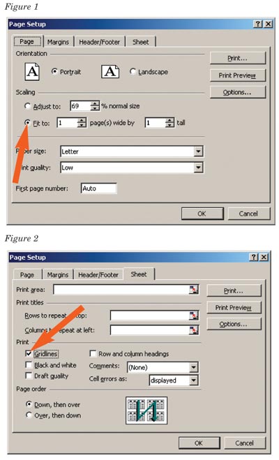
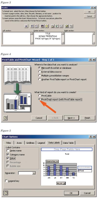
1. Fit to page. On many occasions, I have received spreadsheets that don’t quite fit on one page—they have a bit of information that spills over onto a second page, but only for a few rows or a few columns. If you have a smaller data set, you can often keep the output to one page by using the PAGE SETUP dialogue box (Figure 1). Click on FILE, PAGE SETUP and try the FIT TO 1 page wide by 1 page tall to get a single page printed output. This shrinks the output percentage. While this is useful for minor adjustments, if there is too much data, the printed output might be too tiny for the average reader. You may also be able to slightly tweak the margin settings to keep the printed output to the page. You can also print to a single page wide by multiple pages long. It is a good idea to test the printed output on a page or two to see how it looks. Sometimes, the configuration of the printer itself will limit what actually prints on the paper. 2. Printing gridlines. If you want the printed output to automatically include gridlines, click on FILE, PAGE SETUP, then click on SHEET, then click the GRIDLINES (Figure 2). This can be a timesaver if you don’t need to put special grid coloring, but simply want all data in the printed output to show the grids. In this same dialogue box, you can indicate that you want to see the row and column headings (1, 2, 3, a, b, c, etc.) in the printed output. If your data has column headings, and your printed output has more than one page of text, use the ROWS TO REPEAT at top on the PAGE SETUP - SHEET screen to identify what row will appear at the top row of each printed sheet. Once the dialogue box appears, simply click on the row(s) of the spreadsheet that you want to have repeated on each page. You can use a similar feature for the COLUMNS TO APPEAR AT LEFT so that row headers print on each page.
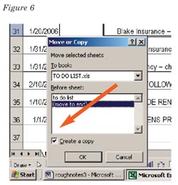
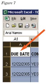
3. Header and footer. Under PAGE SETUP, HEADER/FOOTER you will also find CUSTOM HEADER and CUSTOM FOOTER OPTIONS (Figure 3). This gives you a way to put a specific label at the top or bottom of each printed page, including “page of pages” as well as a date and time of revision, spreadsheet name, worksheet name. If your final audience will be receiving the information on the spreadsheet via e-mail, you may want to consider printing it as a PDF rather than sending the whole spreadsheet. Excel spreadsheets can be rather size-intensive, and creating a digital printed output can often be an easier way to send the information, and it cannot be as easily edited. Charts It is just as easy to create a PivotChart as it is to develop a PivotTable. (PivotTables were discussed in the December 2005 column.) To begin, place your cursor anywhere inside the data set. From the DATA menu click the PIVOTTABLE AND PIVOTCHART REPORT to launch the WIZARD (Figure 4). Select PIVOT CHART REPORT. Once you select “Finish” you will be presented with the chart created from the data. Right click anywhere on the chart to change colors, chart type (bar to pie in an easy click), indicate data labels, and numeric values in the chart itself (Figure 5). Consider providing a “canned version” of the report data to verify your information. Excel is a great tool, but not everyone in your office may know how to utilize the features. Make sure there is a way to locate the “conventional” data source in case there are questions. Other thoughts and comments Formula fields and data fields. If you set up a spreadsheet for others to use in collecting data, and that spreadsheet has formula cells as well as data cells, consider “shading” the cells that contain formulas; then you can instruct the user which cells are for data entry, and which should never be used for data entry (formula cells). You can also use the TOOLS-PROTECTION feature to password protect the spreadsheet from unwanted editing. Another useful tip is to provide the end user with a recap of the formula cells and advise what the result should reveal. For example, if you have data that accumulates premium compared to losses, one cell might contain a formula that calculates a loss ratio. Provide your end users with a “map” and instruction guide for each formula cell.
Keep a copy. If you are an Excel novice, consider copying the active worksheet, either to another page in the workbook, or as an entirely new spreadsheet. Right click on the sheet tab and choose MOVE OR COPY TO make your desired copy option (Figure 6). Choose CREATE A COPY. This is particularly useful if you have a large data sheet. Make a copy of this to a separate workbook so that if something happens to this workbook, you have a starting point. Common challenges Some of the most common challenges in working with Excel are: • Blank data records. When performing functions on a string of contingent cells, make sure you don’t have any gaps in the information. AUTOSUM formula will stop at any blank fields and will add only up to that point. • Selecting too many or not enough cells when sorting. Make sure the selection you want to sort is appropriately identified. If you select only three cells in a single column and choose the A-Z sort option, for example, it will sort only those three cells, not the entire spreadsheet. • Trashed formulas. Make sure you have a guide to the formulas. The most common mistake here is a simple one—people enter data into the formula cell, rendering it useless.
• ###. If you see cells with ###, the cell width is not wide enough to accommodate the largest information set. Place your cursor between the column headers and double click to auto size. TIP: You can auto size an entire worksheet by clicking in the top left block between Row 1 and Column A (Figure 7), which selects all cells in the sheet, then double click between any column header to auto size all cells in the sheet. Words of advice • Know your data. I cannot emphasize enough the importance of understanding your data sources and how your system stores information. Many organizations find they’d be lost without their “Excel guru.” Familiarize yourself with your system’s basic reporting engine first—understand it thoroughly. There are often decent reports available that satisfy many basic reporting needs. Once you understand your system’s basic data structure, the export to Excel or other data tools will only be enhanced. • Know your procedures. Many times, an inaccurate output is not the fault of the data or the system, but the procedures (or lack thereof) in place to collect the data. For example, if you don’t have a consistent method among staff members for collecting data about leads processed and policies issued, you will not be able to get a “success ratio” report. Excel is a marvelous and user-friendly tool, but even a magician cannot pull a non-existent rabbit out of a hat. * The author |
||||
|